How to Unhide Google Sheet Column
In this tutorial, we will learn how to hide and unhide Google Sheet Column
Hide columns and rows from users' views if you want to keep them from wandering into portions of a worksheet you don't want them to see. This approach is commonly used to hide confidential data or calculations, but you may also want to use it to hide underused or unnecessary regions to keep your users' attention on the information that matters.
When changing your own sheets or investigating inherited spreadsheets, on the other hand, you'll want to unhide all rows and columns to see all of the data and comprehend the dependencies. Both possibilities will be explained in this essay.
Google Sheets Unhiding Rows and Columns
Unhide Google Sheet Column: 6 Steps
Step 1 - Open the google sheets app: First of all, we’ll Open the “Google Sheet”. On your mobile device, look for the icon of google sheets. It looks like an A4-size green sheet of paper. It has a white outlined square over it. Further, the square divides into four identical cells. Or we can simply go to the browser’s bar address and type sheets.google.com
Now, we will select the google excel sheet file that we want to sort out. Open that green A4 sheet like looking app. Create a new Google sheet. By clicking on the google sheet.

Step 2 - Click on any column: When you open Google Sheets, you’ll see a list of your sheets. You need to create a new Google Sheet if there is no sheet. Create one or choose the one you want to work on in Google Sheets.
- Now, Click on a column's heading to choose it. You can either choose one column or more than one.
- Drag the mouse across the column headings to pick multiple contiguous columns. Alternatively, select the first column and then choose the last column while holding down the Shift key.
- To pick non-contiguous columns, click the first column's heading and then click the headings of the subsequent columns you wish to choose while holding down the Ctrl key.

Step 3 - Click on the 3 dot option: After selecting the whole column you'll see three dots on your screen. Click on the three dots.
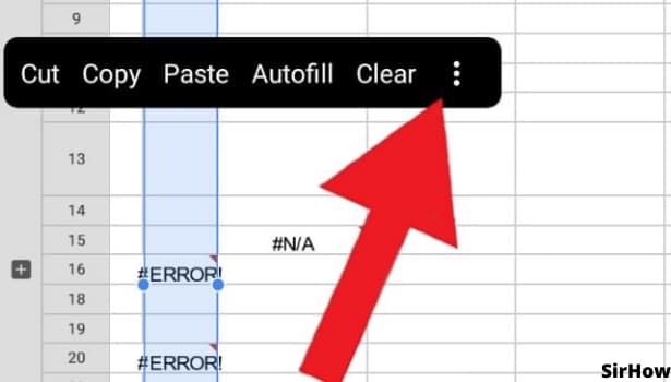
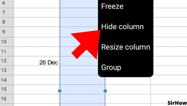
Step 4 - Click on the hidden column: As is the case with nearly all common tasks in Excel, there is more than one way to hide columns. After selecting the whole column click on the right button of the mouse. You'll see a number of options there. Choose "Hide Column".
Shortcut: If you'd rather not take your hands off the keyboard, use this shortcut to rapidly hide the selected row(s): Ctrl + 9 is a combination of the keys Ctrl and 9.
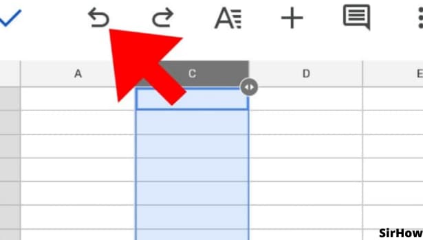
Step 5 - You can see here B column is hidden now: As you can see here that our column B is hidden now. We'll let's unhide it. Shall we? Alright, for that you just need to click on the left arrow to redo that is to unhide.
- You know there are a few different ways to unhide columns in Google sheet.
- Just as there are a few different ways to hide them.
- It's entirely up to you to decide which one to implement.
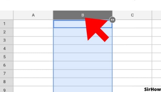
Step 6 - You can see B column is visible again: Viola! Your hidden column is visible again, now you can use this trick anytime and on any excel sheet.
This is how you can hide and unhide columns in Google sheets in a few simple steps.