How to Make Pivot Table in Google Sheets
Just like the other tables and charts, you can also make a pivot table in Google sheets.
It will not take to more than one minute to make a Pivot table in Google sheets. You can organize and make your data/ information look more presentable with the help of pivot tables. So, we would highly recommend learning how to make a Pivot table in sheets with the help of this article. Similarly, you can also insert line graphs in Google sheets.
Google Sheets Pivot Tables
Make Pivot Table in Google Sheets in 5 Steps
Step-1 Open The Google Sheet: It is completely your choice whether you want to open a fresh Google sheet or work on an existing one.
Let us explain to you more:
- If you want to open an existing Google sheet, then you will need the link to that particular Google sheet. After that, you just need to place the link in your web browser and click on search to open it up.
- Or, you can also consider opening the Google sheets website on your web browser if you want to create a new one.

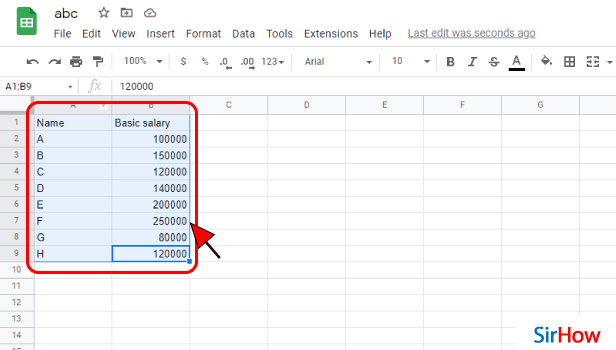
Step-2 Select Your Data/Cells: Then, in this second step, you have to simply select the cell or cells where you have entered your data.
To select the cells/data, just right-click on your mouse while placing it on the first cell. Then, drag it until all your data is selected.
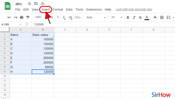
Step-3 Go To The 'Insert' Tab: After you have selected the data, then you have up click on the 'Insert' tab from the very top of your google spreadsheet.
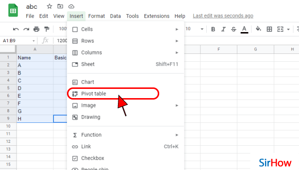
Step-4 Click on 'Pivot Table': In the second section of the list menu, you will find four options. These four options are:
- Chart
- Pivot table
- Image
- Drawing
From here, you have to choose the option of 'Pivot Table'. This is because you want to add this tabel to your sheet.
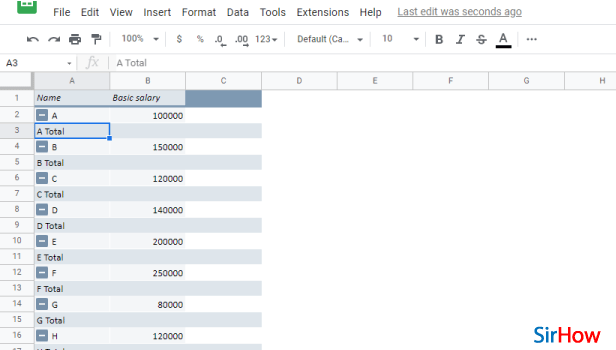
Step-5 Pivot table is Added Now: As you can see in the below picture now, your pivot table has been added where initially there was your data entered simply.
FAQ
How Can I Create a Pivot Table With Multiple Columns in Google Sheets?
You can easily create a private table with multiple columns in your sheets by using the feature known as a pivot table editor.
We have elaborated the steps for you to learn about it further:
- Go to your Google sheet.
- Then, go to the 'pivot table editor.
- And, then you have to click the 'Add' button next to the Rows.
- Then, locate the row you want to show and click on them.
- Now, you can repeat the same process to insert a Column to start seeing your pivot table take shape.
That's all you have to do!
Can I Also Format/Customize a Pivot Table in Google Sheets?
Google sheets provide you with the option to format or customize a pivot table in the Google sheets application.
You can easily adjust the overlap look and format of your pivot table. Along with the format, you can also change the font, fill, number format, and other features. In this way, you can give your pivot table a more neat look.
Is It Possible To Make a Pivot Table with Data From Multiple Sheets Google Sheets?
If you are wondering that would it be possible for you to make a pivot table from data that is spread in multiple Google sheets, then the answer is NO!
- Your data has to be accumulated in a single table only if you want to make a pivot table.
- Another alternative to the situation is, to insert the file that contains your data into your Google sheet. For example, in Google sheets you can insert a pie chart, column chart, line graph, etc.