How To Freeze A Google Sheet Row
When working with enormous datasets in Google Sheets, you'll find yourself scrolling down or to the right frequently. And you might want to have some particular rows and columns displayed while you're doing it, so you can figure out what a data point represents and which row/column you're looking at. To do so, you'll need to use Google Sheets to freeze rows and columns. In this article, we will look at How To Freeze A Google Sheet Row.
How to: Freeze Rows or Columns in Google Sheets
Freeze A Google Sheet Row in 4 Steps
Step 1 - Open Google Sheets App: Google sheet is an excellent tool for content creators. Look for the Google Sheets icon on your mobile device. It appears to be a green A4 sheet of paper with a fold in the top-right corner.
- If you are unable to find the app on your device, go to the Google Play Store and download it.
- In the search field, type 'Google Sheets.' After that, check for the icon that has been described.
- Install Google Sheets and open it after you've found it.

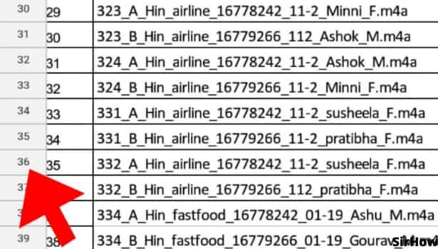
Step 2 - Click on Row Number: Now, you have installed the google sheets app on your device. Open it and go to the spreadsheet in which you want to freeze rows or columns. Now you need to select all the rows or columns which you want to freeze.
- For selecting the row, just click on the row number. Row numbers appear in the extreme left of the row.
- To be sure that the row is selected, look for a blue rectangle covering the row completely.
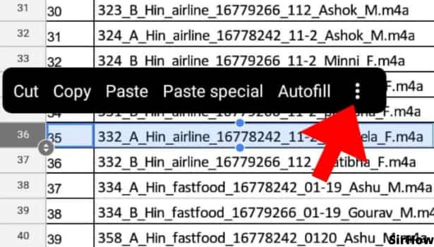
Step 3 - Click on the three Dot Option: After selecting the row or column which you want to freeze, look for the three-dot option. You will need to right-click on the row number (or the column number if you want to freeze a column).
- You will see many options like copy, paste, etc. Tap on the 3 dots option. After clicking on the three dots option, you will have a drop-down menu with many more options to edit the selected row or column.
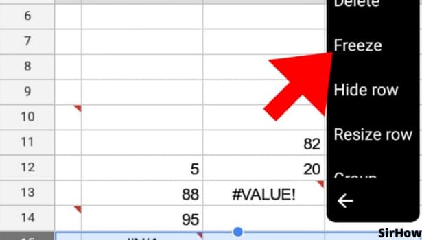
- You have options like hide row, resize row, etc. Navigate through these options and find the freeze option.
- Click on it to freeze the required row
Step 4 - Click on Freeze Option To Freeze Google Sheets Row: After you click on the Freeze Google Sheet Row option, the selected row is frozen. That is, when you scroll up or down, you will always see the frozen row.
- This is extremely helpful in large data set in which all the data does not appear on one page.
- This option is useful when you quickly scroll your spreadsheet down and view a particular row without losing track of what you are looking at.
- This option also lets you quickly scroll back up and resume scrolling smoothly.
In Conclusion
When you freeze rows in Google Sheets, they will remain visible as you navigate down the page. When you freeze columns, they will also become visible when you scroll to the right. This option is useful when you quickly scroll your spreadsheet down and view a particular row without losing track of what you are looking at
Frozen rows will not affect other rows in the Google sheet - they stay put until you unfreeze them. Next time you open your sheet, the frozen row will still be there. You can make changes without affecting any of your formulas.